Anatomy of a Modern Data Pipeline — Five Roles
Last Updated: September 12, 2026
Where this document fits
Understand the roles of Kafka, Spark, Airflow and Flink and the contracts between pipeline components.
Sources, ingestion, storage, processing and consumption are conceptual roles. Products need not perform exactly one role, and every pipeline need not store before processing. Streams can be processed before storage; transformations can run inside a warehouse. Define schema, freshness, retention, replay and output-duplication contracts first.
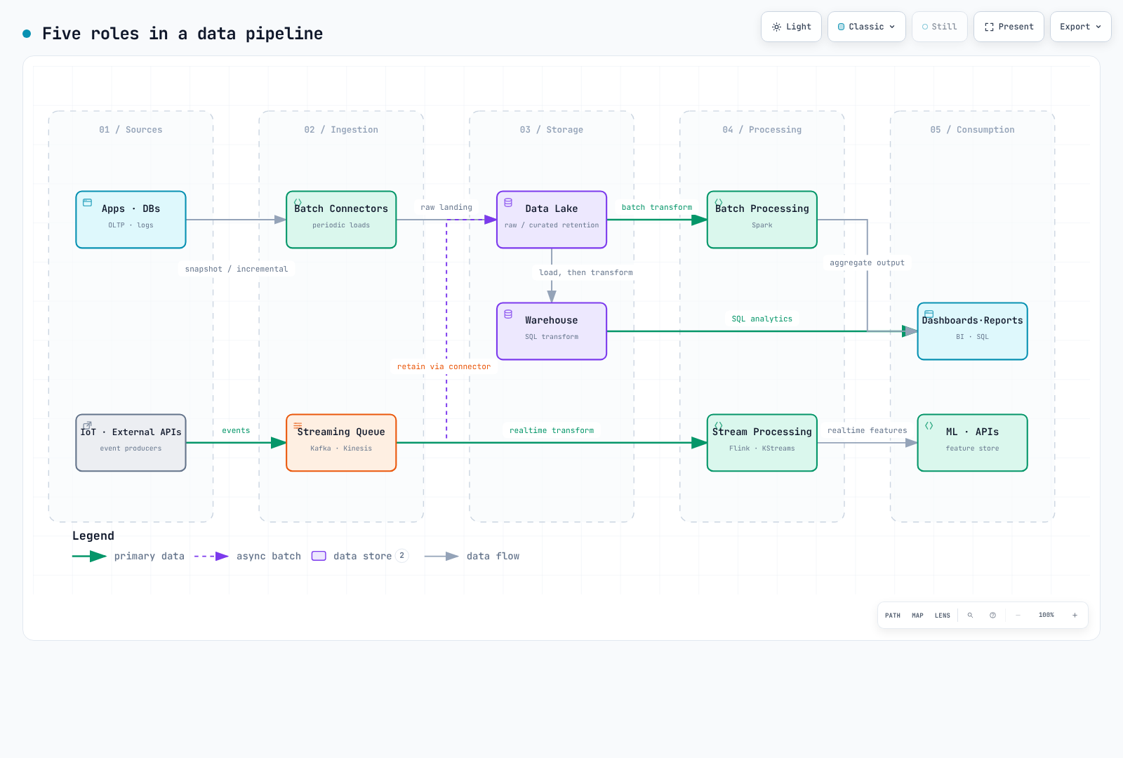
1. Sources — Changes and Load
Sources include application databases, logs, IoT devices and external APIs. Choose full snapshots, incremental queries or log-based CDC as needed. Log-based CDC depends on database replication logs, retention and permissions; schema-change support varies by connector and format.
Read replicas and log-based extraction can reduce production-database load. They are not supported by every database/connector combination. Check initial snapshot load, replication lag and recovery after missing logs.
2. Ingestion — Batches and Events
| Mode | Behavior | Examples | Latency drivers |
|---|---|---|---|
| Batch ingestion | Extract/load groups on a schedule or condition | Airbyte, JDBC batch jobs | Schedule, data volume and destination |
| Event ingestion | Continuously publish and consume changes/events | Kafka, Kinesis, Pulsar | Producer, transport, consumer and sink delays |
Apache Sqoop retired in June 2021, so it is not a new-adoption example. Batch and streaming ingestion may be used separately or together.
Kafka offsets can replay records that still exist. Time/size retention, log compaction and tombstone policies can remove historical events. A retention-duration setting alone does not guarantee a complete event history.
Replay alone does not provide end-to-end exactly-once behavior. Source positions and processing state need consistent recovery, while sink transactions, idempotency and external side effects must follow the same contract. Re-executing a record after failure is different from applying its final effect twice.
The eight Kafka operations chapters and Part 9 benchmark cover the EKS choices.
3. Storage — Originals and Query Models
| Choice | Examples | Design considerations |
|---|---|---|
| Data lake | S3 files/objects | Raw and curated data, retention, access, quality and query cost |
| Warehouse | Redshift, Snowflake, BigQuery | Loading and SQL transformation, tables, performance and governance |
| Lakehouse | Iceberg, Delta Lake, Hudi | Format/engine compatibility, concurrency and maintenance |
Retaining raw data in a lake is useful for replay but is not the only standard path. Reprocessing still requires actual retained data and access.
ETL means extract → transform → load into the destination. ELT means extract → load → transform in the destination. Moving already-curated results into a warehouse is not ELT merely because a warehouse is involved. Using both a lake and warehouse does not determine the transformation order.
4. Processing — Bounded and Continuous Inputs
Spark supports batch processing and Structured Streaming; Flink also processes streams and bounded inputs. Batch/stream classifications do not assign mutually exclusive roles to products.
Possible designs include fast provisional stream results followed by late-data corrections, or batch recomputation for settlement. Streaming is not inherently approximate, and batch is not inherently exact. Event time, watermarks, allowed lateness, deduplication, state/checkpoints and output contracts determine the result.
See the Spark and Flink guides for engine operations.
5. Consumption — Result Contracts
BI, reports, ML feature stores and data APIs consume results. Turn requirements such as “five-minute dashboard lag,” “settlement corrections after close,” or “one-second recommendation-feature target” into measurable contracts. These numbers are examples, not product performance guarantees.
Cross-Cutting Operations
- Orchestration: Tools such as Airflow manage dependencies, schedules and retries for batch-oriented work. They are not engines processing every streaming event, and having two pipelines does not automatically require Airflow.
- Schema contracts: Registry compatibility is enforced in the registration, serialization or CI paths where checks are applied. It does not automatically block every source-database DDL or business-semantic change. Connect compatibility policy with actual consumer tests.
- Observability: Inspect lineage, freshness, missing/duplicate data, quality metrics and recovery history.
Through an EKS Lens
Kafka, Spark and Flink use their respective Operators/deployment models. Airflow uses Helm, executors and task operators such as KubernetesPodOperator. An Airflow “Operator” is not the same concept as a Kubernetes controller. Storage, analytics and managed workspaces can live in external AWS services. Compare ownership with the managed alternatives.
References
The conceptual breakdown began with Abhishek Agrawal's “Anatomy of a Modern Data Pipeline” infographic; the contracts and operating guidance were reviewed separately.