ClickHouse on EKS Measured Benchmark

Recorded Test Environment: ClickHouse 24.8 (as measured — the 24.x series is now end-of-life, see the version note under Test environment), Kubernetes 1.36 (Amazon EKS) Last Updated: September 11, 2026

Every benchmark report says "ClickHouse is fast" — but it's surprisingly hard to find numbers measured on an ordinary EKS node with a default gp3 volume. This document loads 100 million Kubernetes log rows into a deliberately modest environment — a 4 vCPU node and a default-configuration gp3 100 GiB volume — and measures what happens. These are reported historical results. This page does not include the complete original query_log, every exact query or cache state, so identical numbers are not guaranteed. Preserve exact SQL, settings, versions and raw results for the new-run examples below.

Architecture diagram showing the ingest path from the numbers_mt generator into the MergeTree table, and the query path through primary-index pruning, the bloom filter skip index, and column reads served from either the page cache or gp3 directly.Open full screen ↗

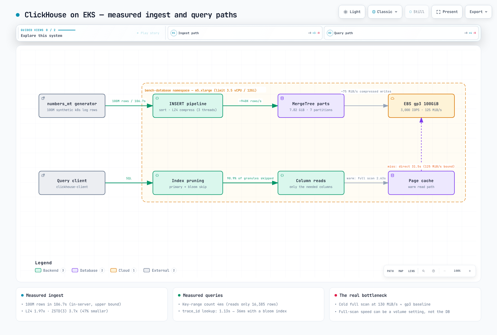
TL;DR — measured results

Measurement	Result
Ingest (in-server generate + insert)	100M rows / 106.7 s = ~940K rows/s
Storage size (LZ4 default)	15.37 GiB → 7.82 GiB (1.97×)
Storage size (ZSTD(3))	15.37 GiB → 4.16 GiB (3.7×), 47% smaller than LZ4
ORDER BY key-range count (1-hour window)	4 ms — counts 59,916 rows while reading only 16,385 of 100M
ERROR count per pod GROUP BY (2-day window)	0.36 s (28M rows scanned)
LIKE '%timeout%' full scan	warm cache 2.63 s / Direct I/O requested 31.5 s (12×)
trace_id point lookup	full scan 1.13 s → 0.036 s with a bloom filter index (31×)

Test environment

Item	Value
Cluster	Amazon EKS, Kubernetes 1.36, ap-northeast-2
Node	m5.xlarge (4 vCPU, 16 GiB) — one dedicated node provisioned by Karpenter (benchmark pod ran alone on it)
Pod resources	requests 2.5 vCPU / 9 Gi, limits 3.5 vCPU / 12 Gi
Storage	EBS gp3 100 GiB, default settings (3,000 IOPS / 125 MiB/s baseline), EBS CSI driver
ClickHouse	official image clickhouse/clickhouse-server:24.8 (24.8.14.39), default configuration
Hourly cost	m5.xlarge on-demand $0.236/h + gp3 100 GiB at $0.0912/GB-month (Seoul region, queried via the Pricing API, 2026-09)

Version note. 24.8 was the LTS release the measurement was taken on, but ClickHouse's security policy no longer lists any 24.x release as supported (as of September 2026 the supported lines are 26.8 LTS, 26.7, 26.6, and 26.3 LTS). Use a current LTS tag for anything new. The mechanisms measured below — primary-key pruning, LZ4/ZSTD codecs, bloom filter skip indexes — are all present in current releases, but re-run the numbers on the version you deploy before using them for sizing.

The environment is intentionally unglamorous. The question this benchmark asks is not "how fast is ClickHouse on a dedicated i-family NVMe box" but "how far do you get on the kind of general-purpose node and default gp3 volume your cluster already has."

Deployment manifest

This rerun example uses supported LTS 26.3.33.24; historical 24.8 measurements remain unchanged. It requires regular EC2 EBS CSI/IAM and PVC provisioning. Preserve the default user's network restriction and benchmark through a localhost client inside kubectl exec. Record the image digest, EBS configuration and actual CPU/memory usage.

apiVersion: v1
kind: Namespace
metadata:
  name: bench-database
---
apiVersion: storage.k8s.io/v1
kind: StorageClass
metadata:
  name: bench-clickhouse-gp3
provisioner: ebs.csi.aws.com
parameters:
  type: gp3
  encrypted: "true"
  iops: "3000"
  throughput: "125"
volumeBindingMode: WaitForFirstConsumer
reclaimPolicy: Delete
---
apiVersion: v1
kind: PersistentVolumeClaim
metadata:
  name: clickhouse-data
  namespace: bench-database
spec:
  accessModes: ["ReadWriteOnce"]
  storageClassName: bench-clickhouse-gp3
  resources:
    requests:
      storage: 100Gi
---
apiVersion: v1
kind: Pod
metadata:
  name: clickhouse
  namespace: bench-database
  annotations:
    karpenter.sh/do-not-disrupt: "true"
spec:
  nodeSelector:
    node.kubernetes.io/instance-type: m5.xlarge
  containers:
    - name: clickhouse
      image: clickhouse/clickhouse-server:26.3.33.24
      resources:
        requests: { cpu: "2500m", memory: 9Gi }
        limits: { cpu: "3500m", memory: 12Gi }
      readinessProbe:
        exec:
          command: ["clickhouse-client", "--host", "127.0.0.1", "--query", "SELECT 1"]
        initialDelaySeconds: 5
        periodSeconds: 5
      volumeMounts:
        - name: data
          mountPath: /var/lib/clickhouse
  volumes:
    - name: data
      persistentVolumeClaim:
        claimName: clickhouse-data

For production lifecycle/recovery automation, one option is a ClickHouseInstallation managed by the Altinity clickhouse-operator rather than a bare Pod. A bare Pod keeps the measurement target simple here.

The dataset — 100 million realistic Kubernetes log rows

Uniform random data (generateRandom) distorts compression ratios, so the rows are generated the way real logs look: repeated templates plus variable fields — 10 namespaces, one pod name per namespace (the pod suffix is hashed from the same bucket that picks the namespace, so there are only 10 distinct pod values — a simplification that matters for the compression numbers, see Measurement 2), a 0.8% ERROR rate, and timestamps spanning 7 days.

CREATE TABLE logs
(
  timestamp   DateTime64(3),
  namespace   LowCardinality(String),
  pod         String,
  container   LowCardinality(String),
  level       LowCardinality(String),
  message     String,
  trace_id    String,
  duration_ms Float32
)
ENGINE = MergeTree
PARTITION BY toDate(timestamp)
ORDER BY (namespace, timestamp);

INSERT INTO logs (timestamp, namespace, pod, container, level, trace_id, duration_ms, message)
WITH
  ['payment','order','user','search','catalog','cart','shipping','auth','gateway','recommend'] AS nss,
  ['GET /api/v1/orders','POST /api/v1/payments','GET /api/v1/users','GET /api/v1/search',
   'POST /api/v1/cart/items','GET /api/v1/products','POST /api/v1/shipments','POST /oauth/token',
   'GET /healthz','GET /api/v1/recommendations'] AS eps
SELECT
  toDateTime64('2026-08-25 00:00:00', 3) + toIntervalMillisecond(number * 6) AS timestamp,
  nss[(cityHash64(number) % 10) + 1] AS namespace,
  concat(namespace, '-7c7dd4f9c-', substring(lower(hex(sipHash64(cityHash64(number) % 10))), 1, 5)) AS pod,
  if(cityHash64(number + 2) % 10 < 8, 'app', 'istio-proxy') AS container,
  multiIf(cityHash64(number + 3) % 1000 < 8, 'ERROR',
          cityHash64(number + 3) % 1000 < 50, 'WARN',
          cityHash64(number + 3) % 1000 < 300, 'DEBUG', 'INFO') AS level,
  lower(hex(sipHash128(number))) AS trace_id,
  round(if(level = 'ERROR', 2000 + (cityHash64(number + 4) % 30000) / 10,
           (cityHash64(number + 4) % 20000) / 100), 1) AS duration_ms,
  multiIf(
    level = 'ERROR', concat('upstream request timeout after ', toString(round(duration_ms)),
                            'ms endpoint=', eps[(cityHash64(number + 5) % 10) + 1],
                            ' status=503 trace_id=', trace_id),
    concat(eps[(cityHash64(number + 5) % 10) + 1], ' completed status=200 in ',
           toString(duration_ms), 'ms trace_id=', trace_id)
  ) AS message
FROM numbers_mt(100000000)
SETTINGS max_threads = 3, max_insert_threads = 2, max_memory_usage = 9000000000;

Measurement 1 — Ingest: 100M rows in 106.7 seconds

Elapsed: 106.747 sec  →  ~936,800 rows/s, 7 daily partitions, 36 active parts

Read this figure for what it is. The rows were generated inside the server and inserted directly (INSERT…SELECT), so network transfer and text parsing costs are absent — it measures an in-server path. It also includes data-generation CPU work, so it is not a mathematical ceiling for external ingestion. Client, format, network, batching and concurrency can change external throughput in either direction. The headline is still real: within a 3.5 vCPU limit, ClickHouse sorted, compressed, and wrote roughly 940K rows per second — on a 125 MiB/s default gp3 volume. Final compressed size divided by elapsed time is about 75 MiB/s, not a measured physical EBS write rate. Check page cache/writeback, merges and durable-flush conditions separately.

Measurement 2 — Compression: which columns spend your money

Overall: 15.37 GiB → 7.82 GiB (1.97×, default LZ4). The per-column breakdown is far more interesting:

Column	Compressed	Uncompressed	Ratio
message	3.97 GiB	8.75 GiB	2.2×
trace_id	3.08 GiB	3.07 GiB	1.0× (incompressible)
timestamp	404.07 MiB	762.94 MiB	1.89×
duration_ms	289.17 MiB	381.47 MiB	1.32×
level	45.88 MiB	95.72 MiB	2.09×
container	39.27 MiB	95.72 MiB	2.44×
pod	9.32 MiB	2.15 GiB	236×
namespace	488.63 KiB	95.72 MiB	201×

Sizes and ratios are exactly as system.parts_columns reported them (formatReadableSize of the compressed/uncompressed byte sums); the ratios are computed from the raw byte counts, not from the rounded sizes.

Two lessons jump out:

1. LowCardinality plus ORDER BY locality is enormous — namespace is the first ORDER BY key, so identical values run in long streaks: 95.7 MiB collapses to 489 KiB. pod compresses 236× for the same reason, with a caveat: this generator emits exactly one pod name per namespace (10 distinct values), so pod behaves like a second copy of namespace. A real cluster, with tens of pods per namespace and new names on every restart, will compress pod noticeably less.
2. High-entropy IDs eat ~40% of your storage — the 32-character hex trace_id barely compressed with LZ4 in this run (1.0×) and accounts for 3.08 GiB of the 7.82 GiB total (39.4%). When you design a log schema, "do we store IDs as strings" is the single biggest storage-cost lever. Hex encodes four bits of information per byte, leaving compression opportunities for other codecs. UUID/FixedString(16) binary representation reduces the raw width, but measure final storage, codec/index effects and query compatibility.

LZ4 vs ZSTD(3) — 47% storage vs 1.9× scans

The same data was re-inserted into a CODEC(ZSTD(3)) table:

	LZ4 (default)	ZSTD(3)
Compressed size	7.82 GiB (1.97×)	4.16 GiB (3.7×)
Re-compression insert (100M rows)	—	120.0 s
LIKE '%timeout%' full scan (warm)	2.63 s	4.9 s

Storage drops 47%, but the CPU-bound full scan slows by 1.9×. LZ4 for hot data plus TTL-driven ZSTD recompression is one option to evaluate. The best codec depends on real data, CPU and I/O constraints.

Measurement 3 — Queries: what is fast, what is slow, and why

Each query ran after dropping the mark/uncompressed caches: ① once with min_bytes_to_use_direct_io=1 to bypass the page cache (Direct I/O requested), ② three warm runs (minimum reported).

#	Query pattern	Direct-to-disk	Warm	Rows read (read_rows)
Q1	WHERE namespace='payment' AND timestamp BETWEEN … (1-hour count)	13 ms	4 ms	16,385 (0.016%) — result 59,916
Q2	ERROR count per pod, 2-day GROUP BY (the LIMIT 10 is trivial here — the dataset has only 10 pods)	0.57 s	0.36 s	28M
Q3	message LIKE '%timeout%' whole-range full scan	31.5 s	2.63 s	100M
Q4	duration p50/p99 per namespace, whole range	1.34 s	1.03 s	100M (no filter)
Q5	trace_id = '…' point lookup (no index)	24.3 s	1.13 s	100M

How to read this:

• Why Q1 is 4 ms: PARTITION BY (day) and ORDER BY (namespace, timestamp) line up, so the one-hour payment window is a single contiguous key range. The query counts 59,916 rows, yet system.query_log shows only 16,385 rows read: since 24.6 ClickHouse counts the granules that lie entirely inside a primary-key range straight from the index and decompresses only the partial granules at the range edges (roughly two granules of 8,192 rows). Verify whether this optimization applies with EXPLAIN indexes = 1 and actual read_rows; it is not unconditional for every count query.
• Q3's 31.5 s (direct) vs 2.63 s (warm): reading the ~4 GiB compressed message column from disk works out to 4 GiB ÷ 31.5 s ≈ 130 MiB/s — pinned in the narrow band where the gp3 volume cap (125 MiB/s) and this m5.xlarge's own EBS baseline (1,150 Mbps ≈ 137 MiB/s) sit; the two limits are too close for this run to say which one bound first. The same query served from the page cache becomes CPU-bound (~38M rows/s). Measured proof that full-scan performance can be a volume-throughput setting, not a database property. (See the EBS gp2 vs gp3 benchmark.) Q5's no-index run tells the same story: 3.08 GiB of trace_id in 24.3 s ≈ 130 MiB/s.
• Why Q4 full-scans 100M rows in ~1 s: column orientation in its purest form — by column size it touches only duration_ms (289 MiB) and namespace (0.5 MiB), not 7.8 GiB, and the warm run is CPU-bound on 100M Float32 quantiles.
• The short Q2/Q4 measurements do not isolate physical disk throughput. A final-size/time ratio above 125 MiB/s does not itself prove a page-cache hit. Dropping mark/uncompressed caches also does not drop the OS page cache. The original run ended before cache/read-method/short-window effects were traced; preserve query_log ProfileEvents together with node/EBS I/O metrics on reruns.

Measurement 4 — bloom filter skip index: 1.13 s → 0.036 s

A trace_id point lookup isn't covered by the ORDER BY key, so by default it's a full scan (1.13 s). Add a skip index:

ALTER TABLE logs ADD INDEX trace_bf trace_id TYPE bloom_filter(0.01) GRANULARITY 4;
ALTER TABLE logs MATERIALIZE INDEX trace_bf;  -- asynchronous; wait for system.mutations.is_done

	No index	bloom_filter(0.01)
Warm lookup time	1.13 s	0.036 s (31×)
Rows read	100M	1.08M (98.9% skipped)
Data read	3.82 GiB	42.6 MiB
Index size	—	119.7 MiB (1.5% of table)

"Jump to a trace ID" is the most common query against an observability log store, and it costs 1.5% extra storage plus a 20-second materialize to get 31×. If you run Grafana on a ClickHouse log backend, evaluate this index against real selectivity, false positives, write/merge costs and query plans.

In cost terms

The 2026-09-11 Pricing API query confirms Seoul Linux m5.xlarge on-demand at $0.236/h and gp3 at $0.0912/GB-month. EBS bills provisioned capacity. Whether the dataset occupies 7.82 or 4.16 GiB, this example's 100 GiB volume costs $9.12/month; $0.71/$0.38 from used bytes is not the actual volume bill.

At 100M rows/day for 30 days, this synthetic LZ4 ratio implies about 235 GiB of data alone. It does not fit the 100 GiB example volume. Add merge workspace, indexes, replicas, backups and headroom when sizing. Provisioning just 235 GiB costs about $21.43/month, before nodes, EKS, networking and operations. Comparing only EBS storage with CloudWatch Logs ingestion does not establish total-cost superiority.

How to reproduce

These are new-run examples for comparing patterns. The exact historical Q1/Q2 windows and Q5 ID are not retained here, so they are not claimed to reproduce the original row counts/timings. Save exact SQL, versions, timezone, read settings and raw results together.

-- Q1: explicit example window for a new run, not recovered historical SQL.
SELECT count() FROM logs
WHERE namespace = 'payment'
  AND timestamp >= toDateTime64('2026-08-26 00:00:00', 3)
  AND timestamp < toDateTime64('2026-08-26 01:00:00', 3);

-- Q2: a two-day example window.
SELECT namespace, pod, count() AS errors FROM logs
WHERE level = 'ERROR'
  AND timestamp >= toDateTime64('2026-08-26 00:00:00', 3)
  AND timestamp < toDateTime64('2026-08-28 00:00:00', 3)
GROUP BY namespace, pod ORDER BY errors DESC LIMIT 10;

-- Q3: full-range message scan.
SELECT count() FROM logs WHERE message LIKE '%timeout%';

-- Q4: approximate quantiles; all candidate rows are still processed.
SELECT namespace, quantiles(0.5, 0.99)(duration_ms) AS p50_p99
FROM logs GROUP BY namespace;

-- Q5: a trace ID that the generator creates for number=42.
SELECT * FROM logs
WHERE trace_id = lower(hex(sipHash128(toUInt64(42))));

kubectl apply -f clickhouse.yaml
kubectl wait -n bench-database pod/clickhouse --for=condition=Ready --timeout=300s
kubectl exec -n bench-database clickhouse -- \
  clickhouse-client --host 127.0.0.1 --query 'SELECT version(), timezone()'
# Save the CREATE TABLE block as schema.sql and INSERT block as insert.sql.
kubectl exec -i -n bench-database clickhouse -- \
  clickhouse-client --host 127.0.0.1 --multiquery < schema.sql
kubectl exec -i -n bench-database clickhouse -- \
  clickhouse-client --host 127.0.0.1 --time --multiquery < insert.sql
# Run the selected query with a unique ID; store its exact SQL with the results.
kubectl exec -i -n bench-database clickhouse -- \
  clickhouse-client --host 127.0.0.1 --query_id benchmark-q3-run1 \
  --time --multiquery < q3.sql

For the Direct I/O requested variant, append SETTINGS min_bytes_to_use_direct_io=1 to that SELECT. Repeat with default read settings and retain every sample plus the median, not only the minimum. After SYSTEM FLUSH LOGS, export matching query_log rows; wait for index materialization in system.mutations before comparison. Record query/filesystem/OS cache and background merge conditions too.

Export results outside the cluster before deleting the dedicated bench-database namespace and bench-clickhouse-gp3 StorageClass. The example's Delete reclaimPolicy deletes benchmark data with the PVC.

Caveats

• Single node, single run environment. Absolute values will differ under replication/sharding or on other instance types. The transferable content is the relative patterns: pruning, column orientation, cache effects, index effects.
• The ingest figure measures in-server generation/insertion, not external collection throughput (see Measurement 1).
• Synthetic-data compression ratios are sensitive to field composition. Including the high-entropy trace_id inside message keeps this conservative, but the pod column (only 10 distinct names, see Measurement 2) is optimistic; real logs may compress better or worse depending on your schema.
• The first warm run is slower while the cache fills (Q3: 8.7 s first, then 2.6 s). Warm values in the tables are the minimum of three runs.

Related reading

• ClickHouse as a log backend — integration with collection pipelines (Fluent Bit/Vector)
• EBS gp2 vs gp3 Measured Benchmark — volume/instance throughput limits relevant to interpreting Q3
• Databases on Kubernetes Overview — the operator landscape and managed vs self-hosted decision framework

Review Sources

• ClickHouse support policy
• Official Docker image behavior
• Quantile sampling
• Data skipping indexes
• Partial count optimization
• EBS pricing